Toon Glass Shader Breakdown

Intro

This shader produces a toon glass effect, which involves solid diagonal lines across the quad’s surface which move with the camera’s position. This is similar to how glass and window reflections are sometimes portrayed in cartoons/comics/clipart etc.

(Note : This blog post uses a different version than in the original tweet above, but the result is very similar)

Notes

• This is an Unlit shader. Transparent surface mode and Alpha blending.
• AlphaClipThreshold should be set to 0 as we don’t want to discard any pixels.
• While this is mostly written for URP, I’ve also tested it in HDRP (High Definition Render Pipeline). I’m using Absolute World below so that the graph can be identical in both pipelines and function correctly. However, I recommend converting this to World when using HDRP. This then allows us to remove the need to subtract the camera’s position, as world positions in the HDRP are already Camera Relative.

Breakdown

Properties

Before we begin the graph, let’s define a bunch of properties. This is done in the Blackboard window, press the “+” icon, choose the type and then right-click to rename the property. The default values can be set under the Node Settings tab of the Graph Inspector window while the property is selected. These defaults will help your previews look the same as mine.

• Color “Colour” – Default : White (255,255,255) with 20 alpha.
• Vector1 “Offset” – Default : 0.2
• Vector1 “Scale Multiplier” – Default : 0.7
• Vector1 “A” – Default : 3
• Vector1 “B” – Default : 1
• Vector1 “Line Width” – Default : 0.5
• Vector1 “Line Alpha” – Default : 0.4

Note that on the actual Material, I’ve changed some of these settings (Offset of 1 and a Scale Multiplier of 0.3). These values look nice in scene, but won’t look good in the shadergraph previews!

I also haven’t named the “A” and “B” properties very well, but they both control the number of diagonal lines produced by the shader. However A also affects how small the lines are in the center while B is more linear. The line count (per side) is equal to A*B.

There is probably a better way to handle this mathematically but what I ended up with worked well enough for me. For best results, B should remain an integer. A doesn’t have to be an integer, but A*B should be. So, A=2.5 and B=2 is fine, for 5 lines per side. A=5 and B=1 would also give 5 lines per side, but the width of the lines would be different.

Breakdown

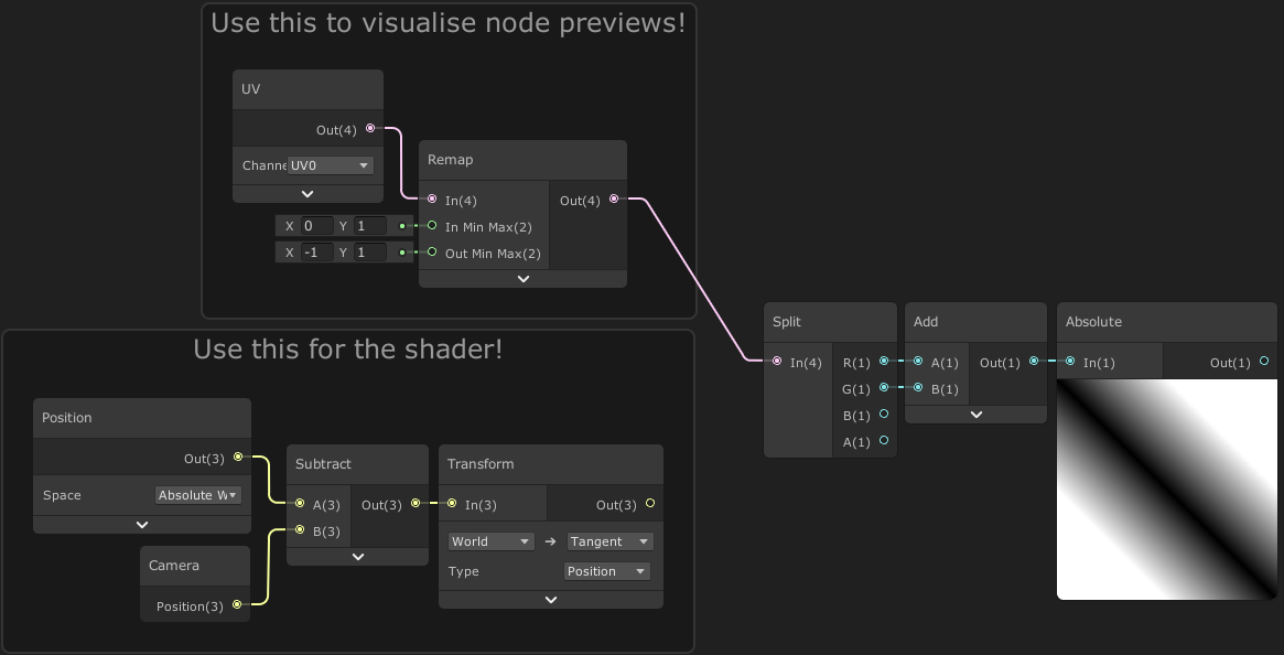
First we create a Position node set to Absolute World space, and Subtract the camera’s position (in world space, via the Position output on the Camera node) to obtain the position relative to the camera. The origin of the effect will now be at the camera’s position so it will move as the camera moves (in terms of translation, not rotation).

We can then Transform to Tangent space, which appears to make the position relative to the meshes’ surface – kind of? Well, at least for our purposes the R/X component of the position is horizontal across the surface, and G/Y is vertical, but there may be better ways of handling this.

We can Split to obtain values for each axis individually, and Add them together to make a diagonal gradient. An Absolute function will then convert any negative values to positive. Any changes made will now be mirrored across the diagonal line as both sides share the same values.

The preview on our Absolute node looks like a sphere which can make things a bit harder to visualise here.

For older versions of Shader Graph, can temporarily use a UV node and put it into a Remap node with values of 0 and 1 for the In Min Max and -1 and 1 for the Out Min Max. This remaps the values so the value at the center of the preview has a value of 0 to closer match the other coordinates we have. When we connect this to the Split we can visualise the previews properly which will help a lot when creating the rest of the graph, then at the end we can reconnect the other position instead.

We now have two gradients going outwards diagonally in each direction. There are values of 0 in the center shown by the black areas on the preview. If we Subtract a value from this it will shift the values inwards, and output negative values in the center (which we can remove later via a Saturate). This results in creating a spacing between the two gradients. Here we use the Offset property, which will allow us to change the spacing later in the inspector. We can then also apply some scaling by using a Multiply with the Scale Multiplier property, as shown on the left below.

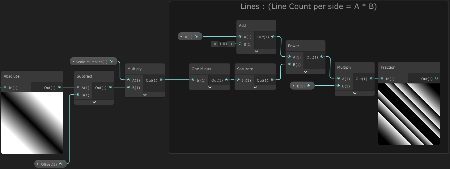
To handle creating multiple lines, I’m using this setup as shown above. By using a Power in our calculations, we can allow the values to be more exponential / less linear, which affects the width of each line based on the distance from the diagonal (as shown in the Fraction node preview).

To possibly better show how this works, I’ve plotted the functions of Power (^x) and Fraction (frac) here :

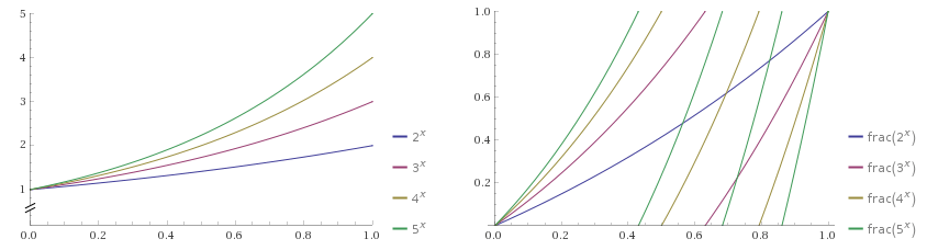
(Source : Wolfram|Alpha, Wolfram Alpha LLC, Date : 01/01/2020, Links : Plot1, Plot2)

Both plots show the “A” property set to 0 to 4 and “B” set to 1. It can be a little messy with the overlapping lines, but try to focus on one at a time. Note that the input on the Power is A+1.01, which I’ve rounded to A+1.

Looking at the plot on the left, When A is higher, the plot results in a more curved line. This should make sense if you’re familiar with powers/exponentials, but the important thing is what happens when putting this through the other function.

The Fraction node returns the fractional (decimal) part of the number (without the integer component). This results in values only between 0 and 1, shown on the right plot. The line jumps from 1 back to 0 on the Y axis. The more curved lines from the previous plot produce more line sections.

We use a One Minus node on our second input on the Power, so that we input values near 1 on diagonal line rather than 0, resulting in smaller width gradients rather than larger.

There’s also a Saturate in place which clamps values between 0 and 1. The extra .01 on the Add node is in place to prevent the Fraction node outputting 1 in the center (the spacing created by the Offset) for certain integer values of A, although it can still occur if B or A*B isn’t an integer, hence the mention of setting these to integers at the start of the breakdown. We could instead mask that area to always be black, but it felt a bit unnecessary.

Finally we can Step the gradient-like result from the Fraction node, using the Line Width property to obtain solid lines which we can then Multiply by our Line Alpha. We also need to Add the Color property’s alpha, to control the glass’ surface alpha, then put this into the Alpha input on the Master node, and also set the Color input as shown.

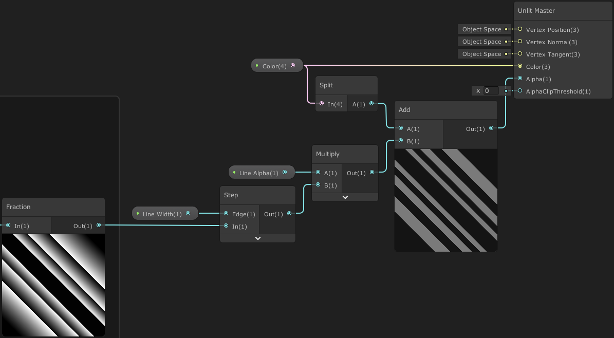
Don’t forget to reconnect our tangent Position coordinates as well if you’re using the UV for visualising/2D previews.

Join my discord! 💬